1.2 Chromatographic Theory
All chromatographic systems have a mobile phase that transports the analytes through the column and a stationary phase coated onto the column or on the resin beads in the column. The stationary phase loosely interacts with each analyte based on its chemical structure, resulting in the separation of each analyte as a function of time spent in the separation column. The less analytes interact with the stationary phase, the faster they are transported through the system. The reverse is true for less mobile analytes that have stronger interactions. Thus, the many analytes in a sample are identified by retention time in the system for a given set of conditions. In GC, these conditions include the gas (mobile phase) pressure, flow rate, linear velocity, and temperature of the separation column. In HPLC, the mobile phase (liquid) pressure, flow rate, linear velocity, and the polarity of the mobile phase all affect a compounds’ retention time. An illustration of retention time is shown in Figure 1.2. The equation at the top of the figure will be discussed later during our mathematic development of chromatography theory.
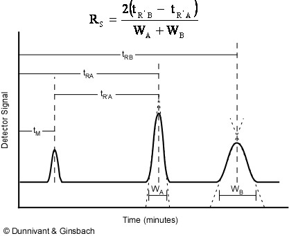
Figure 1.2. Identification of Analytes by Retention Time.
In the above figure, the minimum time that a non-retained chemical species will remain in the system is tM. All compounds will reside in the injector, column, and detector for at least this long. Any affinity for the stationary phase results in the compound being retained in the column causing it to elute from the column at a time greater than tM. This is represented by the two larger peaks that appear to the right in Figure 1.2, with retention times tRA and tRB. Compound B has more affinity for the stationary phase than compound A because it exited the column last. A net retention (tR’A and tR’B) time can be calculated by subtracting the retention time of the mobile phase(tM) from the peaks retention time (tRA and tRB).
Figure 1.2 also illustrates how peak shape is related to retention time. The widening of peak B is caused by longitudinal diffusion (diffusion of the analyte as the peak moves down the length of the column). This relationship is usually the reason why integration by area, and not height, is utilized. However, compounds eluting at similar retention times will have near identical peak shapes and widths.
A summary of these concepts and data handling techniques is shown in Animation 1.1. Click on the figure to start the animation.
Animation 1.1. Baseline Resolution.
Chromatographic columns adhere by the old adage “like dissolves like” to achieve the separation of a complex mixture of chemicals. Columns are coated with a variety of stationary phases or chemical coatings on the column wall in capillary columns or on the inert column packing in packed columns. When selecting a column’s stationary phase, it is important to select a phase possessing similar intermolecular bonding forces to those characteristic of the analyte. For example, for the separation of a series of alcohols, the stationary should be able to undergo hydrogen bonding with the alcohols. When attempting to separate a mixture of non-polar chemicals such as aliphatic or aromatic hydrocarbons, the column phase should be non-polar (interacting with the analyte via van der Waals forces). Selection of a similar phase with similar intermolecular forces will allow more interaction between the separation column and structurally similar analytes and increase their retention time in the column. This results in a better separation of structurally similar analytes. Specific stationary phases for GC and HPLC will be discussed later in Chapter 2 and 3, respectively.
Derivation of Governing Equations: The development of chromatography theory is a long established science and almost all instrumental texts give nearly exactly the same set of symbols, equations, and derivations. The derivation below follows the same trends that can be found in early texts such as Karger et al. (1973) and Willard et al. (1981), as well as the most recent text by Skoog et al. (2007). The reader should keep two points in mind as they read the following discussion. First, the derived equations establish a relatively simple mathematical basis for the interactions of an analyte between the mobile phase (gas or liquid) and the stationary phase (the coating on a column wall or resin bead). Second, while each equation serves a purpose individually, the relatively long derivation that follows has the ultimate goal of yielding an equation that describes a way to optimize the chromatographic conditions in order to yield maximum separation of a complex mixture of analytes.
To begin, we need to develop several equations relating the movement of a solute through a system to properties of the column, properties of the solute(s) of interest, and mobile phase flow rates. These equations will allow us to predict (1) how long the analyte (the solute) will be in the system (retention time), (2) how well multiple analytes will be separated, (3) what system parameters can be changed to enhance separation of similar analytes. The first parameters to be mathematically defined are flow rate (F) and retention time (tm). Note that “F” has units of cubic volume per time. Retention behavior reflects the distribution of a solute between the mobile and stationary phases. We can easily calculate the volume of stationary phase. In order to calculate the mobile phase flow rate needed to move a solute through the system we must first calculate the flow rate.
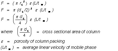
In the equations above, rc is the internal column radius, dc is the internal column diameter, L is the total length of the column, tm is the retention time of a non-retained analyte (one which does not have any interaction with the stationary phase). Porosity (e) for solid spheres (the ratio of the volume of empty pore space to total particle volume) ranges from 0.34 to 0.45, for porous materials ranges from 0.70 to 0.90, and for capillary columns is 1.00. The average linear velocity is represented by u-bar.
The most common parameter measured or reported in chromatography is the retention time of particular analytes. For a non-retained analyte, we can use the retention time (tM) to calculate the volume of mobile phase that was needed to carry the analyte through the system. This quantity is designated as Vm,
![]()
and is called the dead volume. For a retained solute, we calculate the volume of mobile phase needed to move the analyte through the system by
![]()
where tR is the retention time of the analyte.
In actual practice, the analyst does not calculate the volume of the column, but measures the flow rate and the retention time of non-retained and retained analytes. When this is done, note that the retention time not only is the transport time through the detector, but also includes the time spent in the injector! Therefore
![]()
The net volume of mobile phase (V’R) required to move a retained analyte through the system is
![]()
where VR is the volume for the retained analyte and VM is the volume for a nonretained (mobile) analyte.
This can be expanded to
![]()
and dividing by F, yields
![]()
Equation 1.4 is important since it gives the net time required to move a retained analyte through the system (Illustrated in Figure 1.2, above)
Note, for gas chromatography (as opposed to liquid chromatography), the analyst has to be concerned with the compressibility of the gas (mobile phase), which is done by using a compressibility factor, j
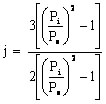
where Pi is the gas pressure at the inlet of the column and Po is the gas pressure at the outlet. The net retention volume (VN) is
![]()
The next concept that must be developed is the partition coefficient (K) which describes the spatial distribution of the analyte molecules between the mobile and stationary phases. When an analyte enters the column, it immediately distributes itself between the stationary and mobile phases. To understand this process, the reader needs to look at an instant in time without any flow of the mobile phase. In this “snap-shot of time” one can calculate the concentration of the analyte in each phase. The ratio of these concentrations is called the equilibrium partition coefficient,
![]()
where Cs is the analyte concentration in the solid phase and CM is the solute concentration in the mobile phase. If the chromatography system is used over analyte concentration ranges where the “K” relationship holds true, then this coefficient governs the distribution of analyte anywhere in the system. For example, a K equal to 1.00 means that the analyte is equally distributed between the mobile and stationary phases. The analyte is actually spread over a zone of the column (discussed later) and the magnitude of K determines the migration rate (and tR) for each analyte (since K describes the interaction with the stationary phase).
Equation 1.3 (V’ R = VR - VM ) relates the mobile phase volume of a non-retained analyte to the volume required to move a retained analyte through the column. K can also be used to describe this difference. As an analyte peak exits the end of the column, half of the analyte is in the mobile phase and half is in the stationary phase. Thus, by definition
![]()
Rearranging and dividing by CM yields
![]()
Now three ways to quantify the net movement of a retained analyte in the column have been derived, Equations 1.2, 1.4, and 1.8.
Now we need to develop the solute partition coefficient ratio, k’ (also knows as the capacity factor), which relates the equilibrium distribution coefficient (K) of an analyte within the column to the thermodynamic properties of the column (and to temperature in GC and mobile phase composition in LC, discussed later). For the entire column, we calculate the ratio of total analyte mass in the stationary phase (CSVS) as compared to the total mass in the mobile phase (CMVM), or
![]()
where VS/VM is sometimes referred to as b, the volumetric phase ratio.
Stated in more practical terms, k’ is the additional time (or volume) a analyte band takes to elute as compared to an unretained analyte divided by the elution time (or volume) of an unretained band, or rearranged, gives
![]()
![]()
where μ is the linear gas velocity and the parameters in Equation 1.10 were defined earlier. So, the retention time of an analyte is related to the partition ratio (k’). Optimal k’ values range from ~1 to ~5 in traditional packed column chromatography, but the analysts can use higher values in capillary column chromatography.
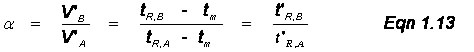
Multiple Analytes: The previous discussions and derivations were concerned with only one analyte and its migration through a chromatographic system. Now we need to describe the relative migration rates of analytes in the column; this is referred to as the selectivity factor, α. Notice Figure 1.2 above had two analytes in the sample and the goal of chromatography is to separate chemically similar compounds. This is possible when their distribution coefficients (Ks) are different. We define the selectivity factor as
![]()
where subscripts A and B represent the values for two different analytes and solute B is more strongly retained. By this definition, α is always greater than 1. Also, if one works through the math, you will note that
The relative retention time, α, depends on two conditions: (1) the nature of the stationary phase, and (2) the column temperature in GC or the solvent gradient in LC. With respect to these, the analyst should always first try to select a stationary phase that has significantly different K values for the analytes. If the compounds still give similar retention times, you can adjust the column temperature ramp in GC or the solvent gradient in LC; this is the general elution problem that will be discussed later.
Appropriate values of α should range from 1.05 to 2.0 but capillary column systems may have greater values.
Now, we finally reach one of our goals of these derivations, an equation that combines the system conditions to define analyte separation in terms of column properties such as column efficiency (H) and the number of separation units (plates, N) in the column (both of these terms will be defined later). As analyte peaks are transported through a column, an individual molecule will undergo many thousands of transfers between each phase. As a result, packets of analytes and the resulting chromatographic peaks will broaden due to physical processes discussed later. This broadening may interfere with “resolution” (the complete separation of adjacent peaks) if their K (or k’) values are close (this will result in an a value close to 1.0). Thus, the analyst needs a way to quantify a column’s ability to separate these adjacent peaks.
First, we will start off with an individual peak and develop a concept called the theoretical plate height, H, which is related to the width of a solute peak at the detector. Referring to Figure 1.2, one can see that chromatographic peaks are Gaussian in shape, can be described by
![]()
where H is the theoretical plate height (related to the width of a peak as it travels through the column), σ is one standard deviation of the bell-shaped peak, and L is the column length. Equation 1.14 is a basic statistical way of using standard deviation to mathematically describe a bell-shaped peak. One standard deviation on each side of the peak contains ~68% of the peak area and it is useful to define the band broadening in terms of the variance, σ2 (the square of the standard deviation, σ). Chromatographers use two standard deviations that are measured in time units (t) based on the base-line width of the peak, such that
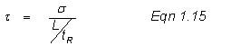
Here, L is given in cm and tR in seconds. Note in Figure 1.2, that the triangulation techniques for determining the base width in time units (t) results in 96% if the area or ±2 standard deviations, or
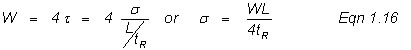
Substitution of Equation 1.16 into Equation 1.14, yields
![]()
H is always given in units of distance and is a measure of the efficiency of the column and the dispersion of a solute in the column. Thus, the lower the H value the better the column in terms of separations (one wants the analyte peak to be as compact as possible with respect to time or distance in the column). Column efficiency is often stated as the number of theoretical plates in a column of known length, or
![]()
This concept of H, theoretical plates comes from the petroleum distillation industry as explained in Animation 1.2 below. Click on the Figure to play the animation.
Animation 1.2 Origin of H and the Theoretical Plate Height Unit
To summarize Animation 1.2 with respect to gas and liquid chromatography, a theoretical plate is the distance in a column needed to achieve baseline separation; the number of theoretical plates is a way of quantifying how well a column will perform.
We now have the basic set of equations for describing analyte movement in chromatography but it still needs to be expanded to more practical applications where two or more analytes are separated. Such an example is illustrated in Animation 1.3 for a packed column.
Animation 1.3 Separation of Two Analytes by Column Chromatography.
Separation of two chemically-similar analytes is characterized mathematically by resolution (Rs), the difference in retention times of these analytes. This equation, shown earlier in Figure 1.2, is
![]()
where tR’B is the corrected retention time of peak B, tR’A is the corrected retention time of peak A, WA is the peak width of peak A in time units and WB is the width of peak B. Since WA = WB = W, Equation 1.19 reduces to
![]()
Equation 1.18 expressed W in terms of N and tR, and substitution of Equation 1.17 into Equation 1.18, yields
![]()
Recall from Equation 1.10, that
![]()
substitution into Equation 1.21 and upon rearrangement, yields
![]()
Recall that we are trying to develop an equation that relates resolution to respective peak separations and although k’ values do this, it is more useful to express the equation in terms of α, where α = k'B / k'A. Substitution of α into Equation 1.22, with rearrangement, yields
![]()
or the analyst can determine the number of plates required for a given separation:
![]()
Thus, the number of plates present in a column can be determined by direct inspection of a chromatogram, where Rs is determined from Equation 1.20, k’A and k’B are determined using Equation 1.10, and α is determined using Equation 1.12.
![]()
![]()
![]()
Another use of Equation 1.23 is that it can be used to explain improved separation with temperature programming of the column in GC and gradient programming in HPLC. Recall that poorer separation will result as peaks broaden as they stay for extended times in the column and several factors contribute to this process. N can be changed by changing the length of the column to increase resolution but this will further increase band broadening. H can be decreased by altering the mobile phase flow rate, the particle size of the packing, the mobile phase viscosity (and thus the diffusion coefficients), and the thickness of the stationary phase film.
To better understand the application of the equations derived above a useful exercise is to calculate all of the column quantification parameters for a specific analysis. The chromatogram below (Figure 1.3) was obtained from a capillary column GC with a flame ionization detector. Separations of hydrocarbons commonly found in auto petroleum were made on a 30-meter long, 0.52-mm diameter DB-1 capillary column. Table 1.1 contains the output from a typical integrator.
Figure 1.3 Integrator Output for the Separation of Hydrocarbons by Capillary Column GC-FID.
Table 1.1 Integrator Output for the Chromatogram shown in Figure 1.3.
| Analyte | Retention Time (min) |
Area Peak |
Width at the Base (in units of minutes) |
|---|---|---|---|
Solvent (tM) |
1.782 |
NA |
NA |
| Benzene | 4.938 |
598833 |
0.099 |
| Iso-octane | 6.505 |
523678 |
0.122 |
| n-Heptane | 6.956 |
482864 |
0.100 |
| Toluene | 9.256 |
598289 |
0.092 |
| Ethyl Benzene | 13.359 |
510009 |
0.090 |
| o-Xylene | 13.724 |
618229 |
0.087 |
| m-Xylene | 14.662 |
623621 |
0.088 |
Example 1.1
Calculate k’, α, Rs, H, and N for any two adjacent compounds in Table 1.1.
Solution:
Using peaks eluting at 13.724 and 13.359 minutes the following values were obtained.

Problem 1.1
Figure 1.4 and Table 1.2 contain data from an HPLC analysis of four s-Triazines (common herbicides). Calculate k’, α, Rs, H, and N for any two adjacent compounds. Compare and contrast the results for the resin packed HPLC column to those of the capillary column in the GC example given above.
Figure 1.4 HPLC Chromatogram of Four Triazines. The analytical column was an 10.0 cm C-18 stainless steel column with 2 μm resin beads.
Table 1.2 Integrator Output for the HPLC Chromatogram shown in Figure 1.4.
| Analyte | Retention Time (min) |
Area |
Peak Width at the Base (in units of minutes) |
|---|---|---|---|
| Solvent (tM) | 1.301 |
NA |
NA |
| Peak 1 | 2.328 |
1753345 |
0.191 |
| Peak 2 | 2.922 |
1521755 |
0.206 |
| Peak 3 | 3.679 |
1505381 |
0.206 |
| Peak 4 | 4.559 |
1476639 |
0.198 |
| Frank's Homepage |
©Dunnivant & Ginsbach, 2008