1.3 Optimization of Chromatographic Conditions
Now we will review and summarize this lengthy derivation and these complicated concepts. Optimization of the conditions of the chromatography system (mobile phase flow rate, stationary phase selection, and column temperature or solvent gradient) are performed to achieve base-line resolution for the most difficult separation in the entire analysis (two adjacent peaks). This process results in symmetrically-shaped peaks that the computer can integrate to obtain a peak (analyte) area or peak height. A series of known reference standards are used to generate a linear calibration line (correlating peak area or height to analyte concentration) for each compound. This line, in turn, is used to estimate the concentration of analyte in unknown samples based on peak area or height.
An instrument’s resolution can be altered by changing the theoretical plate height and the number of theoretical plates in a column. The plate height, as explained in the animation below, is the distance a compound must travel in a column needed to separation two similar analytes. The number of theoretical plates in a column is a normalized measure of how well a column will separate similar analytes.
Now it is necessary to extend the concept of theoretical plate height (H) a bit further to understand its use in chromatography. Since gas and liquid chromatography are dynamic systems (mobile flow through the column), it is necessary to relate a fixed length of the column (the theoretical plate height) to flow rate in the column. Flow rate is measured in terms of linear velocity, or how many centimeters a mobile analyte or carrier gas will travel in a given time (cm/s). The optimization of the relationship between H and linear velocity (μ), referred to as a van Deemter plot, is illustrated in Figure 1.5 for gas chromatography.
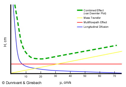
Figure 1.5. A Theoretical van Deemter Plot for a Capillary Column showing the Relationship between Theoretical Plate Height and Linear Velocity.
It is desirable to have the smallest plate height possible, so the maximum number of plates can be “contained” in a column of a given length. Three factors contribute to the effective plate height, H, in the separation column. The first is the longitudinal diffusion, B (represented by the blue line in Figure 1.5) of the analytes that is directly related to the time an analyte spends in the column. When the linear velocity (μ??is high, the analyte will only spend a short time in the column and the resulting plate height will be small. As linear velocity slows, more longitudinal diffusion will cause more peak broadening resulting in less resolution. The second factor is the multi-flow path affect represented by the red line in Figure 1.5. This was a factor in packed columns but has been effectively eliminated when open tubular columns (capillary columns) became the industry standard. Third are the limitations of mass transfer between and within the gas and stationary phases, Cu (the yellow line in Figure 3) defined by
![]()
where μ is the mobile phase linear velocity, Ds and Dm are diffusion coefficients in the stationary and mobile phases respectively, df and dp are the diameter of the packing particles and the thickness of liquid coating on the stationary phase particles respectively, k is the unitless retention or capacity factor, and f(k) and f’(k) are mathematical functions of k.
If the linear velocity of the mobile phase is too high, the entire “packet” of a given analyte will not have time to completely transfer between the mobile and stationary phase or have time to completely move throughout a given phase (phases are coated on the column walls and therefore have a finite thickness). This lack of complete equilibrium of the analyte molecules will result in peak broadening for each peak or skewing of the Gaussian shape. This, in turn, will increase H and decrease resolution.
The green line in Figure 1.5 represents the van Deemter curve, the combined result of the three individual phenomena. Since the optimum operating conditions has the smallest plate height; the flow rate of the GC should be set to the minimum of the van Deemter curve. For gas chromatography this occurs around a linear velocity of 15 to 20 cm/s. However, in older systems, as the oven and column were temperature programmed, the velocity of the gas changed which in turn changed the mobile phase flow rate and the linear velocity. This has been overcome in modern systems with mass flow regulators, instead of pressure regulators, that hold the linear velocity constant.
These concepts are reviewed in Animation 1.4. Click the figure to start the animation.
Animation 1.4 Construction of a van Deemter Curve for an HPLC System
Now that the theoretical basis for understanding chromatographic separation has been established, it is necessary to extend these ideas one step further. Remember, the power of chromatography is the separation of complex mixtures of chemicals; not just for two chemicals as illustrated previously. In most cases separating mixtures of many compounds is required. This requires that the resolution, Rs, be constantly optimized by maintaining H at its minimum value in the van Deemter curve.
This optimization is accomplished by systematically altering the column temperature in GC or the solvent composition in HPLC. Analytes in the separation column spend their time either “dissolved” in the stationary phase or vaporized in the mobile phase. When analytes are in the stationary phase they are not moving through the system and are present in a narrow band in the length of the column or resin coating. As the oven temperature is increased, each unique analyte has a point where it enters the mobile phase and starts to move down the column. In GC, analytes with low boiling points will move down the column at lower temperatures, exit the system, and be quantified. As the temperature is slowly increased, more and more analytes (with higher boiling points) likewise exit the system. In reverse-phase HPLC, analytes with more polarity will travel fastest and less polar analytes will begin to move as the polarity of the mobile phase is decreased. Thus, the true power of GC separation is achieved by increasing the oven/column temperature (referred to as ramping) while in LC the separation power is in gradient programming (composition of the mobile phase). This is “the general elution problem” that is solved by optimizing the mobile phase, linear velocity, and the type of stationary phase. As noted, temperature programming is used to achieve separation of large numbers of analytes in GC. An example of the effects of temperature programming on resolution is illustrated in Figure 1.6. In Figure 1.6a, a low isothermal temperature is used to separate a mixture of six analytes with limited success as some peaks contain more than one analyte. A higher isothermal temperature, shown in Figure 1.6b, is more successful for analytes with higher boiling points but causes a loss of resolution for peaks that were resolved at the lower isothermal temperature. The temperature program used to produce Figure 1.6c achieves adequate separation and good peak shape for a complex solution.
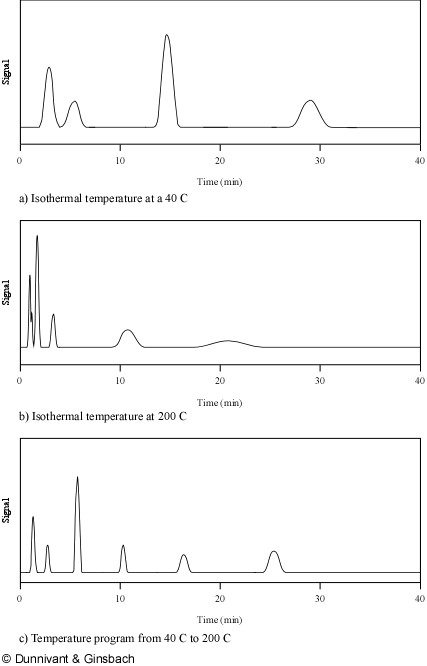
Figure 1.6. Temperature Programming: The Solution to the General Elution Problem for GC Applications.
| Frank's Homepage |
©Dunnivant & Ginsbach, 2008